ThermoLib

Description

ThermoLib is an open-source Matlab/C library for computation of thermodynamic properties (enthalpy, entropy and volume) based on DIPPR correlations for ideal mixtures and on cubic equations of state for real mixtures (e.g. Peng-Robinson or Soave-Redlich-Kwong). The main purpose of the library is to provide first and second order derivatives of thermodynamic functions necessary in process simulation, model predictive process control and vapor-liquid equilibrium computations. The library requires access to substance data from the DIPPR database.

Important note

The routine LoadParams, which is necessary for using any ThermoLib routine, converts igHF and igS from kJ/kmol to J/kmol and Pc from atm to Pa. However, the current version of the DIPPR database already provides the values of these properties in J/kmol and Pa. Consequently, the ThermoLib routines will return incorrect values of the thermodynamic properties if you are using a version of the DIPPR database where igHF and igS are already in J/kmol and Pc is in Pa. This issue will be fixed in the next version of ThermoLib. However, we also describe how you can fix this yourself if you do not want to wait for the next version.

In order to fix the Matlab interface of ThermoLib, you should remove *1000.0 from line 102 and 105 and remove *P0par from line 156 of <path-to-library>/matlab/util/common/LoadParams.m.

In order to fix the C interface of ThermoLib, you should remove 1e3* from the two places that it appears in line 85 of <path-to-library>/matlab/util/common/InstallData.m. Furthermore, you should remove *P0 from line 168 of <path-to-library/src/util/common/LoadParams.c.

Thanks to Arjan van Mulukom for pointing out this issue to us.

Downloads

The newest version of ThermoLib (v. 1.1.7) presents a number of updates and bug fixes:

• A synopsis has been added to all C documentation pages
• The C documentation pages displayed incorrect description of sizes of input arrays (missing squares). This has been fixed
• Several Matlab documentation pages (and help pages) have been fixed
• The parameter array obtained from LoadParams must now be larger
• A function (NoPar) has been added which returns the number of elements in the array obtained from LoadParams in order to ease memory allocation
• The settings file in <path-to-library>/settings/settings.mk now includes paths to MEX compilers
• Header files now include external "C" {} statements to ensure compatibility with C++ code

Documentation pages for the most recent version are available here

• ThermoLib v. 1.1.7 documentation pages

A technical report describing the thermodynamic model that is implemented in ThermoLib is available here

• ThermoLib technical report

Previous version of ThermoLib documentation pages may be downloaded here

• ThermoLib v. 1.1.4 documentation pages
• ThermoLib v. 1.0.0 documentation pages

Prerequisities

ThermoLib relies on data from the DIPPR database, however, the data is not distributed with ThermoLib. The DIPPR 801 Database can be purchased/downloaded here. DIPPR distribute their data in a Microsoft Access database. The data needs to be processed in order to be used within ThermoLib. As much as possible of the transformation has been automated but it does require some manual action by the user. The entire process is described below. The process is described for Microsoft Access 2010. The procedure might be different for other versions of Microsoft Access.

Transformation of data

We need to extract the following four tables from the Microsoft Access database (.mdb file)

• DIPPR CONSTANTS
• Ideal Gas Heat Capacity
• Liquid Density
• Vapor Pressure

Follow the steps below to manually export the DIPPR data to text files and produce data files compatible with ThermoLib

1. Open the Microsoft Access database
2. For each of the above four tables do the following
   • Double click the table name in the left overview
   • Click the pane External Data in the top menu
   • Press the button Text File in the export panel
   • In the menu that appears
     • Under File Name: choose <path-to-library/matlab/data/MicrosoftAccess>
     • Check the box Export data with formatting and layout
     • Click Ok
     • Choose Windows (default)
     • Click Ok
     • Click Close
3. Navigate to the folder <path-to-library/matlab/data>
4. Run the script InstallData.m from Matlab/Octave

After completing these steps, the script InstallData.m should have produced the files

• DIPPRdata.mat: for use with the Matlab/Mex part of ThermoLib
• DIPPRdata.dat: for use with the C part of the library

In order to verify that data is loaded correctly you may run the Matlab script ConductUnitTests.m as follows

1. Navigate to the folder <path-to-library/matlab/test>
2. Run the script ConductUnitTests.m from Matlab/Octave Compares output of all library functions to stored reference values

If data has been loaded as expected and if the Matlab library is correct, the script will produce a list of Matlab function names each followed by ".. success".

NOTE: The script InstallData.m can be rather slow on Windows machines.

Installation

Matlab installation

The Matlab part of ThermoLib requires no installation in particular. Once the DIPPR data has been installed as discussed above, you should simply run the script LoadLibrary.m which is located in the top level of ThermoLib.

1. Run the loading script: LoadLibrary.m from Matlab/Octave
   • adds absolute paths to Matlabs search path

C installation

The C part of ThermoLib is installed by means of a makefile. The procedure is as follows

1. Open a terminal
2. Navigate to the top level folder in ThermoLib
3. Run configuration script. Checks if all prerequisities are installed and if data is located correctly.

    ./configure
   

4. Compile library. Compiles source code into static and dynamic libraries.

    make
   

5. Optional: Install library to system. Moves the compiled libraries to </usr/local/lib/thermolib>, and header files to </usr/local/include/thermolib>.

    make install
   

6. Optional: Run unit tests. Evaluates all C library functions and checks if they produce expected results.

    make ut
   

NOTE: If in doubt, try make help to see what functionality is available.

NOTE: Both make install and make uninstall require super-user privileges.

Mex installation

The installation of Mex files for Matlab and Octave is carried out using the same makefile as above. The procedure is as follows

1. Open a terminal
2. Navigate to the top level folder in ThermoLib
3. Run configuration script. Checks if all prerequisities are installed and if data is located correctly.

    ./configure
   

4. Compile library and mex files. Compiles Matlab/Octave gateway functions into .mexa64/.mex files that can be called from Matlab/Octave.

    make mex
   

NOTE: The installation of the Mex files does not require installation of the C part in advance. It will automatically make a local installation of the C library if necessary.

Matlab tutorials

We consider the chemical species benzene, toluene and diphenyl. As we will see, benzene and toluene are more similar to each other than they are with diphenyl. We will compute liquid properties at temperature $T^l = 425\,\text{K}$ and vapor properties at $T^v = 850\,\text{K}$. Except for the case of ideal mixtures, we compute properties at a pressure of $P = 35\,\text{Bar}$. Because of limitations in the correlations used for ideal liquid properties, we consider a pressure of $P = 5\,\text{Bar}$ for ideal mixtures.

We want to compute both pure component properties and the properties of a mixture of the three species. Furthermore, we want to know their properties both when they are assumed to be ideal and when their properties are computed using a cubic equation of state (Peng-Robinson). In summary, we consider benzene, toluene and diphenyl as

1. Ideal pure components
2. An ideal mixture
3. Real pure components
4. A real mixture

Ideal pure components

First we need to load data from the DIPPR library. Benzene, toluene and diphenyl have the indices 232, 233 and 324 in the database, respectively. Next, we specify the temperatures and the pressure and use the functions PureIdVapHSV and PureIdLiqHSV to compute the molar pure component vapor and liquid properties, respectively

% Specify the desired components (benzene, toluene, diphenyl)
comp = [232, 233, 324];

% DIPPR parameters and sizes
params = LoadParams(comp);

% Specify the desired temperatures and pressure
Tl = 425;  % K
Tv = 850;  % K
P  = 35e5; % Pa

% Compute molar vapor (h, s, v) for each pure component
[hv, sv, vv] = PureIdVapHSV(Tv, P, params);

% Compute molar liquid (h, s, v) for each pure component
[hl, sl, vl] = PureIdLiqHSV(Tl, P, params);

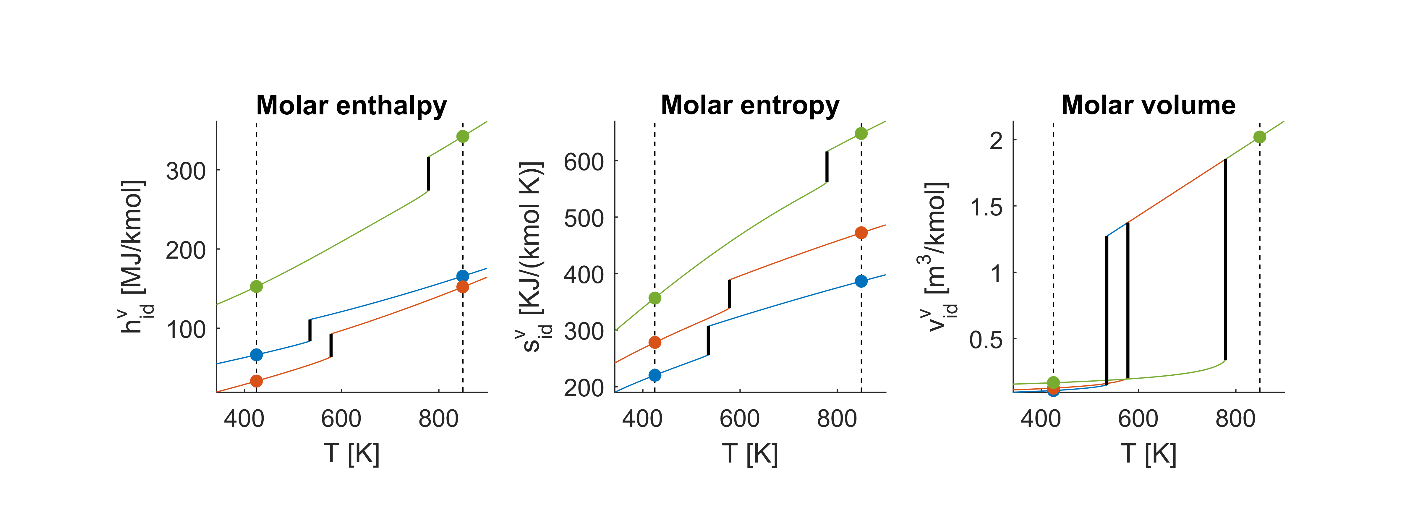
The figure below shows the thermodynamic properties for a range of temperatures at constant pressure $P=35\,\text{Bar}$. Blue lines indicate benzene, red lines indicate toluene and green is diphenyl. The boiling points are marked with black horizontal lines. We see that the boiling point of diphenyl is significantly higher than that of the other two. The properties computed just above are marked with dots.

Real pure components

We now repeat the above computations without assuming ideality. Instead we use the Peng-Robinson equation of state to compute residual properties and thus real pure component properties. We load parameters as above except that we also specify that we would like to load Peng-Robinson cubic equation of state parameters as well. Next, we use PureRealVapHSV and PureRealLiqHSV to compute the molar pure component vapor-liquid properties, respectively

% Specify the desired components (benzene, toluene, diphenyl)
comp = [232, 233, 324];

% DIPPR parameters and sizes
params = LoadParams(comp, 'PR');

% Specify the desired temperatures and pressure
Tl = 425;  % K
Tv = 850;  % K
P  = 35e5; % Pa

% Compute molar vapor (h, s, v) for each pure component
[hv, sv, vv] = PureRealVapHSV(Tv, P, params);

% Compute molar liquid (h, s, v) for each pure component
[hl, sl, vl] = PureRealLiqHSV(Tl, P, params);

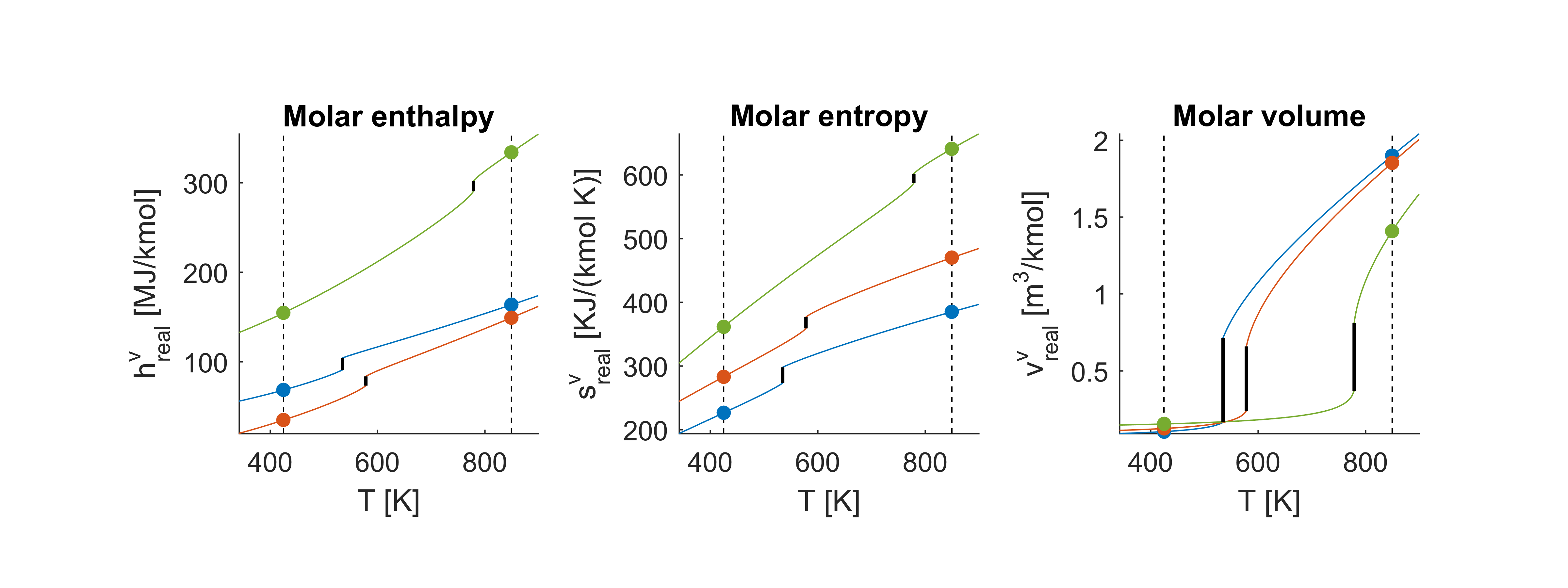
The figure below shows the thermodynamic properties for a range of temperatures at constant pressure $P=35\,\text{Bar}$. As before, blue lines indicate benzene, red lines indicate toluene and green lines are diphenyl, and the properties computed just above are marked with dots. We see that the difference in the properties before and after vaporization is significantly smaller than it was for the ideal properties. In the ideal case, the vapor volume is independent of the component in consideration which is not the case in the figure below.

Ideal mixture

We now consider an ideal mixture of benzene, toluene and diphenyl. Again, we load parameters with LoadParams. Because of limitations in the range of validity of the DIPPR saturation pressure and liquid volume correlations in combination with the two-phase region, we now consider a pressure of $P=5\,\text{Bar}$ instead of $P=35\,\text{Bar}$ as above. The mixture consists of $n = \{6\,\text{kmol}, 4\,\text{kmol}, 5\,\text{kmol}\}$ of benzene, toluene and diphenyl, respectively. We use the functions MixIdVapHSV and MixIdLiqHSV to compute the vapor and liquid properties, respectively

% Specify the desired components (benzene, toluene, diphenyl)
comp = [232, 233, 324];

% DIPPR parameters and sizes
params = LoadParams(comp);

% Specify the desired temperatures and pressure
Tl = 425;  % K
Tv = 850;  % K
P  = 5e5; % Pa

% Specify the desired vapor moles numbers
n = [6; 4; 5]; % kmol

% Compute vapor (H, S, V) for mixture
[Hv, Sv, Vv] = MixIdVapHSV(Tv, P, n, params);

% Compute liquid (H, S, V) for mixture
[Hl, Sl, Vl] = MixIdLiqHSV(Tl, P, n, params);

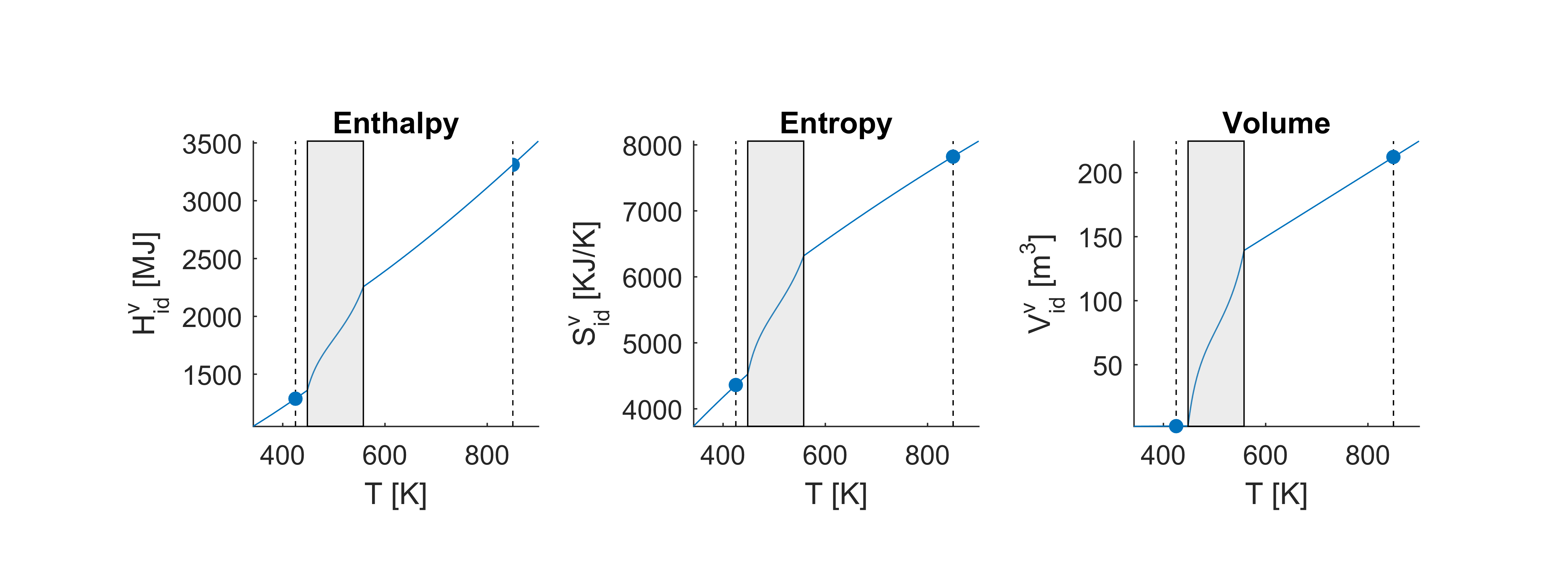
The figure below shows the thermodynamic properties for a range of temperatures at constant pressure $P=5\,\text{Bar}$. Again, the properties computed just above are marked with dots. The shaded box shows the two-phase region of the mixture. We see that much of the complex thermodynamic behavior occurs in the two-phase region and that at higher or lower temperatures, the assumption of ideality makes the thermodynamic properties behave as close to linear. The behavior of the thermodynamic properties in the two-phase region is constructed with the aid of vapor-liquid equilibrium algorithms that are not present in the thermodynamic library

Real mixture

We again consider a mixture of benzene, toluene and diphenyl. We use the Peng-Robinson equation of state to compute residual and thus real mixture properties. We assume that params has been set as in the above tutorials. The mixture again consists of $n = \{6\,\text{kmol}, 4\,\text{kmol}, 5\,\text{kmol}\}$ of benzene, toluene and diphenyl. We specify the van der Waals mixing rule parameters as a symmetric $3\times3$ matrix with all zeros (since the mixture is composed of hydrocarbons). We again use LoadEquationOfState but this time we also provide the mixing rule parameters as inputs. Next, we use MixRealVapHSV and MixRealLiqHSV to compute the mixture vapor-liquid properties, respectively

% Specify the desired components (benzene, toluene, diphenyl)
comp = [232, 233, 324];

% Specify the desired temperatures and pressure
Tl = 425;  % K
Tv = 850;  % K
P  = 35e5; % Pa

% Specify the desired vapor moles numbers
n = [6; 4; 5]; % kmol

% Specify mixing rule parameters
k = zeros(3, 3);

% Load Peng-Robinson (PR) equation of state parameters
params = LoadParams(comp, 'PR', k);

% Compute vapor (H, S, V) for mixture
[Hv, Sv, Vv] = MixRealVapHSV(Tv, P, n, params);

% Compute liquid (H, S, V) for mixture
[Hl, Sl, Vl] = MixRealLiqHSV(Tl, P, n, params);

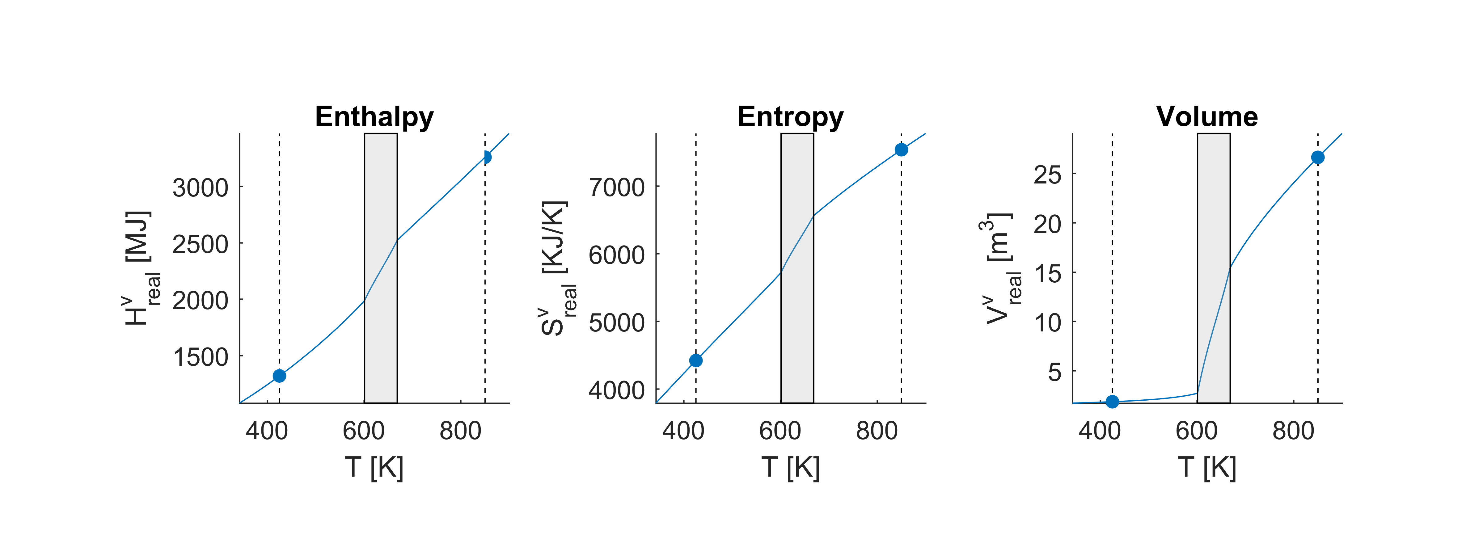
The figure below shows thermodynamic properties for a range of temperatures at constant pressure $P=35\,\text{Bar}$. The properties computed just above are marked with dots. The shaded box shows the two-phase region of the mixture. The real thermodynamic properties are very much similar to the ideal properties for $P=5\,\text{Bar}$ and we can therefore see that increasing the pressure makes the region more narrow and shifts it towards higher temperatures. It should again be noted that the equilibrium algorithms used to produce these figures are not present in the thermodynamic library

NOTE: If you have compiled the Matlab/Octave interfaces you can repeat the Matlab tutorials above by appending Mex to the names of the Matlab routines. parameters must still be loaded with LoadParams.

C tutorial

We will now present a C program that computes the same properties at above. We will decompose the program into parts and discuss each part. The first part is inclusion of headers. We will include the general header ThermoLib.h which contains all other headers.

#include <ThermoLib.h>

Next, we declare i which is simply an auxiliary variable, and we use the variable EquationOfState to specify that we would like to use the Peng-Robinson equation of state. We define temperature, pressure and mole numbers as well as the components of interest, and we allocate memory for the outputs. We will use the variable NumberOfOutputs to specify that we do not want to compute derivatives in this program. This variable is a manual analogue of Matlabs function nargout.

int main(){
    /* Initialization */
    int i;

    /* Equation of state (SRK = 0, PR = 1) */
    int EquationOfState = 1;

    /* Composition (Benzene, Toluene and Diphenyl) */
    int NC = 3;
    int comp[3] = {232, 233, 324};

    /* Temperature, pressure and compositions */
    double Tv = 850;  // K
    double Tl = 425;  // K
    double P  = 35e5; // Pa
    double P2 =  5e5; // Pa
    double n[3] = {6, 4, 5}; // kmol

    /* Thermodynamic outputs */
    double hvid  [NC], svid  [NC], vvid  [NC], hlid  [NC], slid  [NC], vlid  [NC];
    double hvreal[NC], svreal[NC], vvreal[NC], hlreal[NC], slreal[NC], vlreal[NC];
    double Hvid,       Svid,       Vvid,       Hlid,       Slid,       Vlid;
    double Hvreal,     Svreal,     Vvreal,     Hlreal,     Slreal,     Vlreal;

    /* Number of output arguments */
    int NoOutputArguments = 3;

In the Matlab tutorials, we did not discuss tolerances and maximum number of iterations for solving the equations of state. In this program we choose the values below, which are also the default values. The default values can also be chosen with the C library by setting tol and itmax to -1.

    /* Newton parameters */
    double tol = 1e-6;
    int itmax = 40;

The C library is constructed such that the user handles memory allocation. This is in order to avoid unnecessary overhead when the functions are being called repeatedly. First we allocate memory for the parameter array p (called params in the Matlab tutorials). It should always have $12 + 30N_C + N_C^2$ entries of double precision, where $N_C$ is the number of components. Furthermore, each library function will require an array for auxiliary memory which is used internally in the function. Here, we allocate enough auxiliary memory for computation of the thermodynamic functions, but no derivatives. Consult the documentation files to see how much memory is required for computation of first and second order derivatives.

    /* Allocate memory for parameters */
    double p[12 + 30*NC + NC*NC];

    /* Auxiliary memory */
    double memaux_pureidvap[ 2*NC];
    double memaux_pureidliq[11*NC];
    double memaux_mixidvap [ 5*NC];
    double memaux_mixidliq [16*NC];
    double memaux_purereal [13*NC];
    double memaux_mixreal  [15*NC];

Next, we allocate memory for the van der Waals mixing rule parameters and set them all to zero. The DIPPR and equation of state parameters are loaded into the array p using the function LoadParams. These are the last preparations before the actual computations.

    /* Mixing rule parameters */
    double k[NC*NC];

    /* Mixing rule parameters */
    for(i=0; i < NC*NC; i++)
        k[i] = 0.0;

    /* Load parameters (from file) */
    LoadParams(comp, NC, EquationOfState, k, p);

We are now ready to evaluate the C library functions in order to compute the thermodynamic functions as in the tutorials above. The code below will call each of the eight functions that computes the properties of interest. The interfaces are analogous to those of the corresponding Matlab functions, however, the C functions requires an integer containing the number of output arguments together with the auxiliary memory allocated above. After the auxiliary memory input comes the outputs. These should all be pointers such that the function can alter the value. Many of the inputs in the below example are NULL because we do not compute derivatives in this example. Consult the documentation to see how much memory to allocate for the derivative outputs.

    /* Compute vapor thermodynamic functions */
    PureIdVapHSV(Tv, P, p, NoOutputArguments, memaux_pureidvap,
         hvid, svid, vvid, NULL, NULL, NULL, NULL, NULL, NULL, NULL,
         NULL, NULL, NULL);

    PureRealVapHSV(Tv, P, p, tol, itmax, NoOutputArguments, memaux_purereal,
         hvreal,  svreal,  vvreal, NULL, NULL, NULL, NULL, NULL, NULL,
         NULL,    NULL,    NULL,   NULL, NULL, NULL, NULL, NULL, NULL);

    MixIdVapHSV(Tv, P2, n, p, NoOutputArguments, memaux_mixidvap,
        &Hvid, &Svid, &Vvid, NULL, NULL, NULL, NULL, NULL, NULL);

    MixRealVapHSV(Tv, P, n, p, tol, itmax, NoOutputArguments, memaux_mixreal,
        &Hvreal, &Svreal, &Vvreal, NULL, NULL, NULL, NULL, NULL, NULL);

Next are the corresponding liquid properties

    /* Compute liquid thermodynamic functions */
    PureIdLiqHSV(Tl, P, p, NoOutputArguments, memaux_pureidliq,
         hlid, slid, vlid, NULL, NULL, NULL, NULL, NULL, NULL, NULL,
         NULL, NULL, NULL);

    PureRealLiqHSV(Tl, P, p, tol, itmax, NoOutputArguments, memaux_purereal,
         hlreal,  slreal,  vlreal, NULL, NULL, NULL, NULL, NULL, NULL,
         NULL,    NULL,    NULL,   NULL, NULL, NULL, NULL, NULL, NULL);

    MixIdLiqHSV(Tl, P2, n, p, NoOutputArguments, memaux_mixidliq,
        &Hlid, &Slid, &Vlid, NULL, NULL, NULL, NULL, NULL, NULL);

    MixRealLiqHSV(Tl, P, n, p, tol, itmax, NoOutputArguments, memaux_mixreal,
        &Hlreal, &Slreal, &Vlreal, NULL, NULL, NULL, NULL, NULL, NULL);

And finally we terminate the program and return success (0).

    return 0;
}

Compilation

Performance test

The figure below shows a comparison of Matlab, Mex and C code efficiency (left column) as well as a test of the Matlab code with regard to number of components (right column). We see that the Mex code is more than one order of magnitude faster than the Matlab code and the C code is around two orders of magnitude faster. From the top right figure, we see that the Matlab computation time is not very sensitive to the number of components which is most likely due to the efficiency of vectorized computations in Matlab. The C code shows a much more linear tendency with respect to the number of components.

Authors

ThermoLib is created and maintained by Tobias Ritschel, Jozsef Gaspar, Andrea Capolei and John Bagterp Jørgensen, Department of Applied Mathematics and Computer Science & Center for Energy Resources Engineering, the Technical University of Denmark. It has been created as part of several projects and is made available in the hope that it can be useful to others. Feedback, bug reports and suggestions for improvements may be directed to e-mail: info@psetools.org.